
An Optimal Image Packing Algorithm
22 October 2023
Python Implementation
The Rectangle Packing Problem
Arranging images on a canvas to minimize wasted space is a variant of the rectangle packing problem. You have rectangles of different sizes and need to fit them into a larger rectangle efficiently. Game developers deal with this constantly when building texture atlases—packing sprites into a single image cuts down draw calls and speeds up rendering.
The problem is NP-hard. No polynomial-time algorithm exists, and computation time explodes as input grows. Many algorithms exist; none solve it perfectly.
Two-Stage Optimization
The approach here splits the problem into two stages: find the right canvas size, then place the images.
Stage 1: Canvas Size via Binary Search
Binary search finds the smallest canvas that fits all images. The search targets square-ish dimensions because they tend to pack better.
When images don’t fit at a given size, the algorithm removes the largest one and retries. This fallback prevents the search from getting stuck.
def find_optimal_canvas(pictures, ...):
    ...
    return best_canvas_width, best_canvas_height, best_solution

def solve_optimal_arrangement(pictures, ...):
    ...
    return solution
Stage 2: Placement via Constraint Programming
Once the canvas size is fixed, constraint programming handles placement. Images can also be scaled within bounds—sometimes shrinking one image by 5% opens up space that saves 20% overall.
Tools: OR-Tools
OR-Tools is Google’s open-source optimization suite. It handles the constraint satisfaction here.
from ortools.sat.python import cp_model
model = cp_model.CpModel()
solver = cp_model.CpSolver()
Constraints and Objectives
Constraints:
- Boundary: Images stay inside the canvas
- Non-overlapping: No two images share pixels
- Scaling: Images resize within allowed bounds
def add_non_overlapping_constraints(model, x, y, widths, heights):
    ...

def solve_optimal_arrangement(pictures, ...):
    ...
    # Keep images within canvas bounds
    for i in range(n):
        model.Add(x[i] + scaled_widths[i] <= canvas_width)
        model.Add(y[i] + scaled_heights[i] <= canvas_height)
    ...
Objective Functions:
- Unused Space: Minimize empty canvas area
- Max Dimension: Minimize the larger of width/height
- Perimeter: Minimize width + height
-
Squareness: Minimize width - height
def solve_optimal_arrangement(pictures, ...):
    ...
    if objective_type == "unused_space":
        ...
    elif objective_type == "max_dimension":
        ...
    elif objective_type == "perimeter":
        ...
    elif objective_type == "diff_width_height":
        ...
    else:
        raise ValueError("Invalid objective_type.")
    ...
Binary Search Details
The canvas size search doesn’t step down linearly. Binary search over the dimension range converges faster—O(log n) vs O(n) probes.
def find_optimal_canvas(pictures,
initial_canvas_width=INITIAL_CANVAS_WIDTH, initial_canvas_height=INITIAL_CANVAS_HEIGHT, objective_type="perimeter"):
    ...
    while canvas_width_low <= canvas_width_high and canvas_height_low <= canvas_height_high:
        canvas_width_mid = (canvas_width_low + canvas_width_high) // 2
        canvas_height_mid = (canvas_height_low + canvas_height_high) // 2
        ...
Dynamic Scaling Bounds
Scaling factors (alpha values) adjust based on how much space is available. Large canvases allow less scaling; tight canvases allow more. This keeps the solver from wasting time on impossible configurations.
def adjust_alpha_range(picture: tuple, bounding_box_area: float, base_alpha_range: tuple = (BASE_ALPHA_MIN, BASE_ALPHA_MAX)):
    ...
    adjusted_alpha_min = base_alpha_range[0] + 10 * ((area_ratio > 0.8) - (area_ratio < 0.2))
    ...
Initial Arrangement Heuristic
Images are sorted by area, largest first. Placing big images early gives the solver a better starting point than random placement.
def optimized_initial_arrangement(pictures):
    ...
    sorted_pictures = sorted(pictures, key=lambda pic: pic[0]*pic[1], reverse=True)
    return sorted_pictures
Parallel Solving
OR-Tools supports multi-threaded search. On multi-core machines, this speeds up finding solutions.
def solve_optimal_arrangement(pictures, ... , num_search_workers=8, ...):
    ...
    solver = cp_model.CpSolver()
    solver.parameters.num_search_workers = num_search_workers
    ...
Results
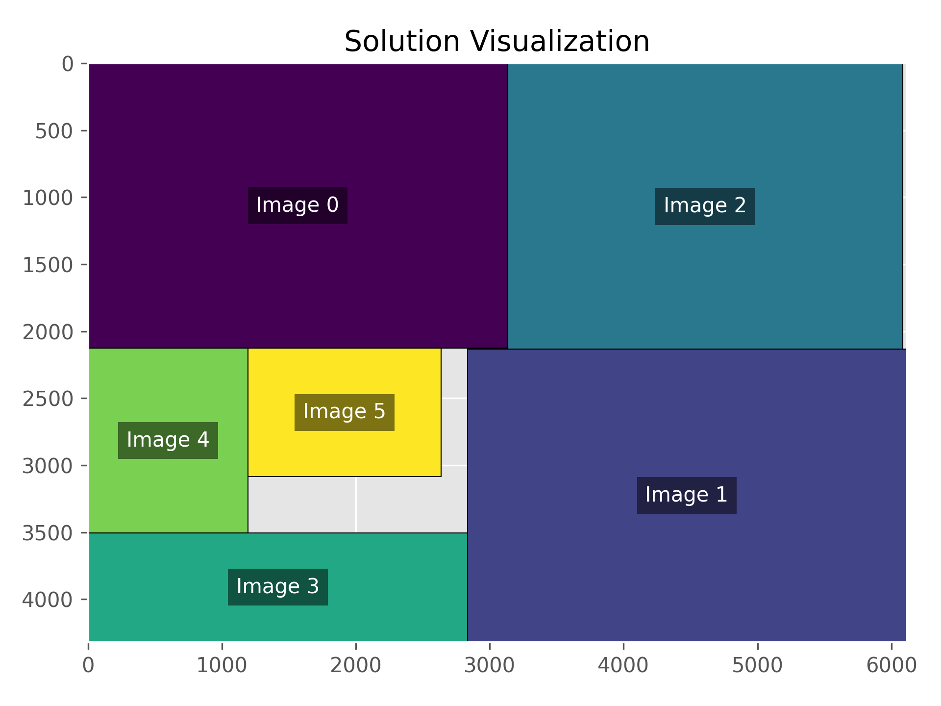
Optimization Log
Using initial picture dimensions: : [(3133, 2126), (2532, 721), (2983, 2156), (961, 640), (980, 1132), (3149, 2102)]
Initial canvas size:           : 8000x8000
Optimized picture arrangement: : [(3133, 2126), (3149, 2102), (2983, 2156), (2532, 721), (980, 1132), (961, 640)]
Trying canvas dimensions:      : 4480x4320. Solution found: No
Trying canvas dimensions:      : 6240x4320. Solution found: Yes
Trying canvas dimensions:      : 5360x4320. Solution found: No
Trying canvas dimensions:      : 5800x4320. Solution found: No
Trying canvas dimensions:      : 6020x4320. Solution found: No
Trying canvas dimensions:      : 6130x4320. Solution found: Yes
Trying canvas dimensions:      : 6075x4320. Solution found: No
Trying canvas dimensions:      : 6102x4320. Solution found: No
Trying canvas dimensions:      : 6116x4320. Solution found: Yes
Trying canvas dimensions:      : 6109x4320. Solution found: No
Trying canvas dimensions:      : 6112x4320. Solution found: No
Trying canvas dimensions:      : 6114x4320. Solution found: No
Trying canvas dimensions:      : 6115x4320. Solution found: No
Optimal canvas dimensions:     : 6116x4320
Adjusted Alpha Below Minimum for Image Size : 2532x721
Area Ratio                     : 0.07
Adjusted Alpha Range           : (70, 150)
Bounding Box Area              : 26421120
Adjusted Alpha Below Minimum for Image Size : 980x1132
Area Ratio                     : 0.04
Adjusted Alpha Range           : (70, 150)
Bounding Box Area              : 26421120
Adjusted Alpha Below Minimum for Image Size : 961x640
Area Ratio                     : 0.02
Adjusted Alpha Range           : (70, 150)
Bounding Box Area              : 26421120
Alpha/Scaling factor for Image 0 : 100%
Alpha/Scaling factor for Image 1 : 104%
Alpha/Scaling factor for Image 2 : 99%
Alpha/Scaling factor for Image 3 : 112%
Alpha/Scaling factor for Image 4 : 122%
Alpha/Scaling factor for Image 5 : 150%